Complex Data Visualisation Made Easy with R and ggplot2 – Course Materials

A CHI 2022 course

Welcome!

Welcome to this CHI 2022 course! I am delighted that you have decided to learn more about creating high quality visualisations in a predictable declarative way. This page contains the course materials. If you are looking for general information about the course, take a look at the course page. You can refer back to these materials at your convenience. I hope you enjoy the course and find it useful and stimulating.

Sandy Gould, course tutor

Session overview

There are two parts to this session

• A quick introduction to ggplot2 and the benefits of taking a declarative approach to visualization
• A practical activity where you will have a go at building a visualization using ggplot2.

Slides

Please feel free to follow along with a copy of the slides.

Software

For this course we will be using software called RStudio. This is a popular tool for writing scripts in R. We’re going to use a browser-based version of RStudio. When the course starts, you should head to https://rstudio.sjjg.uk with the credentials that you have been given.

The RStudio instance I hosted was only available while the course was running. You’ll need to download and install RStudio on your computer (it’s free), and download the package of files that you’ll need for the exercises.

First plot

The goal is that you build-up the visualisations from first principles. If you get stuck though, there’s another R script called visuals-full.R. If you open this, it contains the finished version of each plot.

Getting our data

We’re going to be using data about the countries authors have in their primary affiliations in CHI 2022 papers. These are stored in a chi22-country.csv file.

Note that country names have been adjusted to fit easily with R’s mapping libraries. This means that some countries do not have their full legal names. I apologise for this, I have done so only to keep the task more straightforward.

In the Files pane in the bottom right, select the visuals.R file. This will load the file in the Editor pane in the top left. The top few lines of this file read:

#Import ggplot2 and other useful ready-made code
library("tidyverse")

#Import our 2022 country data
chi22 <- read.csv2("chi22-country.csv",sep=",")

Select these lines (That first line imports ggplot2 along with some other data wrangling tools that we’re going to need later on.) and then click the ‘Run’ button at the top of the pane:

That will load the data from that spreadsheet into a variable. You can see it in the environment view:

If you click the little table icon on the right-hand side of that pane, then it will show you the data table.

Doing the plot

Now you have some data, we can start thinking about plotting something. Underneath the lines to import the CHI 2022 data file, you will see these lines:

Plot 1 is a very simple plot:

ggplot(data = chi22, mapping = aes(x=Country, y=Pubs)) + 
    geom_point()

Note that the + symbol tells R that the statement to create the visualisation has been split over another line. Without them the lines would get very very long!

Everything is a bit squashed though – there’s not enough room on our x-axis for our left-to-right English text. The easiest way to fix this is to tell R to flip the two axes around. To do this, we just have to add an additional function call to our plot declaration:

ggplot(data = chi22, mapping = aes(x=Country, y=Pubs)) + 
    geom_point() +
    coord_flip()

coord_flip() allow us to continue to build our visualisation in the most ’logical’ way, treating the issue of the left-right nature of English as something to be solved with an aesthetic rotation.

If you’re wondering why you can’t just swap the x and y variable in the aes() function around… give it a go! It will work just fine for this kind of plot but for others that expect categories on the x-axis and continuous variables on the y-axis it will cause some plotting problems.

Getting some order to proceedings

Now you should have a plot that is vaguely readable. The order of countries on the y-axis isn’t ideal, though. It’s in reverse alphabetical order, instead of ranked by number of publications. We can make a simple change to our code. We just substitute the Country in our x=Country part of the aes() function for a reordered version of this list. We can reorder it using the reorder() function. We tell this function which column we want to reorder and then what we want to order it by. As we want to reorder our Country list based on the count of Pubs. So we swap x=Country for x=reorder(Country, Pubs):

ggplot(data = chi22, mapping = aes(x=reorder(Country, Pubs), y=Pubs)) +
  geom_point() +
  coord_flip()

If you run that line you’ll end up with something like this:

Tidying up with titles and subtitles

Our plot isn’t perfect. First, our axis labels don’t make any sense. Let’s try and fix them. We can ‘add’ the lab() (i.e., labels) method to our existing plot. We’re going to add a title, subtitle and axes labels. ggplot2 lets us ‘stack’ functions, so we can build up our visualization.

ggplot(data = chi22, mapping = aes(x=reorder(Country, Pubs), y=Pubs)) +
  geom_point() +
  coord_flip() +
  labs(x="Number of CHI 2022 Publications", 
       y="Country",
       title="CHI 2022 Publictions",
       subtitle="Papers track")

That’s better. It’s a little bit dull at the moment, but it does the job. We’ll come back to changing appearance later on.

Trying different geometries

So far we’ve looked at using geom_point as our ggplot2 geometry. There are a lot of other kinds of geometry. Some are suitable for the kind of data we have (one continuous variable, publication count; one discrete variable, country). There is an excellent guide for which geometries might best serve your data. For us, it might also be worth looking at a few other geometries. Let’s try using geom_col() instead of geom_point().

Try just editing your existing plot so that instead of

geom_point() +

it instead reads

geom_col() +

That was easy, wasn’t it? We’ve gone from a point-based plot to a column-based one. It’s showing exactly the same data, of course, but this kind of simple control will become more useful when we move to more complex designs of chart in the next section.

Extension activity

If you have time, try using some other kinds of geometry for this data. What works? What doesn’t?

Can you get geom_text() working? You need to supply a label parameter to it. You can ‘stack’ geometries in a single plot. Try adding multiple geometries to your plot.

Controlling the appearance of plots

Now we have a plot of reasonable quality. It’s fairly minimalist and is of publication quality. But one of the nice things about taking a declarative approach to visualisation is that you can start to develop a ‘house style’ for your visualisations. You can see an example of a ‘house style’ on The Economist, which is known for its distinctively styled graphics.

ggplot2 allows you to customize the look and feel of your graphics in a few ways.

• Appearance as part of aesthetics
• Appearance as part of geometries
• Appearance as part of theming

We’ll come on to appearance as part of aesthetics in the next part of the class. For now, we’ll focus on appearance as part of geometries and theming.

Appearance as part of geometries

A very simple way to change colours is through geometries. In other words, we make the colour part of the drawing of the shapes that are being used to create our visualisation.

So far, the geometry part of our plots has been a bit plain. Either it’s been:

geom_point() +

or

geom_col() +

Going back to our latest version that uses geom_point() we can make a couple of simple changes to alter the appearance of the points (because changing geom_point() will only change the points, nothing else about the plot). We’re going to change the points so that they are orange and make them a little bigger:

ggplot(data = chi22, mapping = aes(x=reorder(Country, Pubs), y=Pubs)) +
  geom_point(colour="Orange", size=3) +
  coord_flip()

Feel free to re-add the labels to your plot if you prefer things to look tidy!

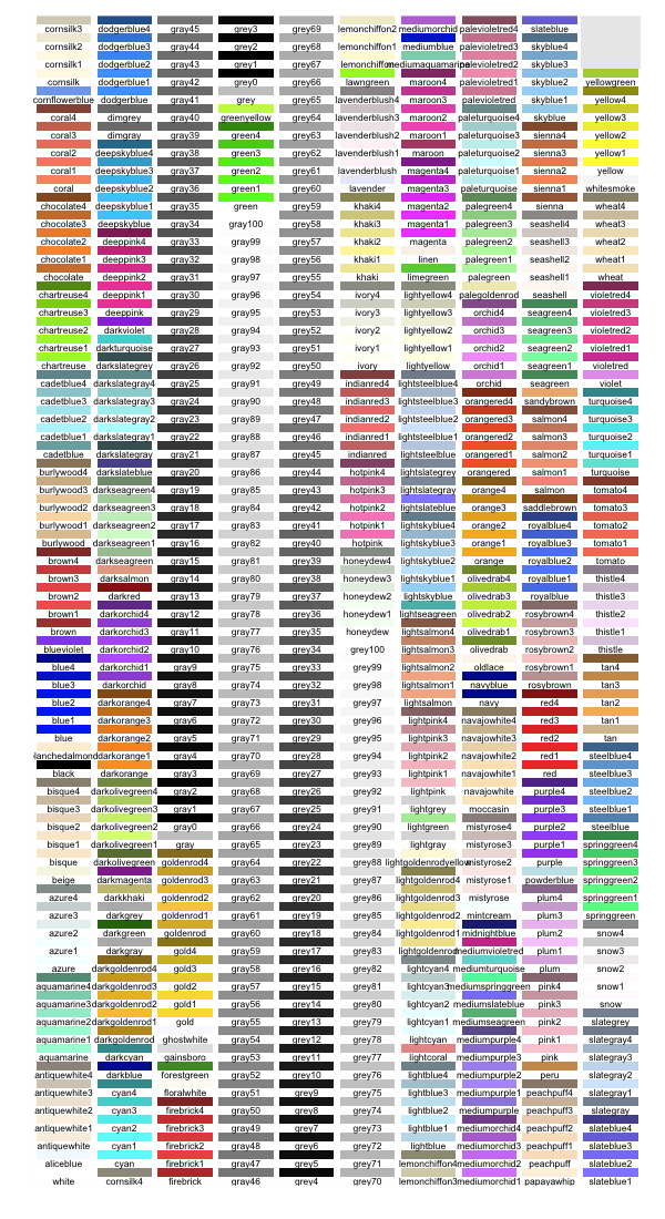
Have a go at playing around with different colours and point sizes. There is a helpful list of the ‘built-in’ colours. You can use these, or, if they are familiar to you, you can also use HTML-style colours instead, for instance:

geom_point(colour="#a3116d",size=3) +

Going back to our geom_col() example, things are a bit more complicated. Try adjusting your plot to replace your geom_point() with geom_col(). Things aren’t looking quite right. That’s because the colour parameter of geom_col() changes the colour of the outline of the rectangles. To change the colour of the whole bar, we need to use the fill parameter instead. So change colour to fill. The size of the bars is automatically computed for geom_col(). So we can remove the size argument too.

So, we can quite quickly change the appearance of our plot by manipulating the geometry (i.e., the ‘how’ of what gets plotted, rather than the ‘what’ of what gets plotted). This will only control the appearance of the geometry we have set it for though. Nothing about the rest of the plot.

To control the appearance of the plot more generally we can use themes.

Controlling appearance using themes

We have looked at aesthetics and geometries so far. These define what will be visualised and how it will be drawn. To control the appearance of plots in a more general sense, things like fonts, gridlines, axes and legends we can use ggplot2 themes. ggplot2 comes with a large number of built in themes. We’re going to use these to begin with, and then we’re going to try customising things.

To our last plot using geom_point() we need to add an extra line:

coord_flip() +
theme_dark()

theme_dark() is a built-in theme. You should instantly notice a change in how things look! Try some of the other built in themes, theme_light() and theme_minimal(). This simple change has a big difference on the overall appearance of the visualisation, but the what (aesthetic) and the how (geometry) of the visualisation has not changed.

Making theme changes yourself

We’re going to make some changes to the theme. To do that, make sure that you are using the theme_minimal() theme, as this is a handy place to start.

We’re going to adjust the theme using the theme() function. This allows us to manipulate all sorts of aspects, from the printing of legends to the ticks on the axes to the orientation of fonts. We’re going to keep things simple, though by:

• Changing the colour and size of the major x-axis gridlines.
• Removing all other gridlines
• Changing the size and colour of the x-axis labels

To do this, we first need to add a theme method to our last plot:

ggplot(data = chi22, mapping = aes(x=reorder(Country, Pubs), y=Pubs)) +
  geom_point(colour="Orange",size=3) +
  coord_flip() +
  theme_minimal() +
  theme()

Now we’re going to populate this theme. To do this, we supply a number of options as parameters to the theme() function. The first one we’re going to add is panel.grid.major.x. This controls the major gridlines on the x-axis. panel.grid.major.x tells ggplot2 what we want to change. To tell it how we want to change it, we need to pass something to this parameter. One of the elements that ggplot2 plots are made from is lines. We can access line objects through the element_line() method. This all sounds complicated, but it’s quite straightforward. Change the last line to:

theme(panel.grid.major.x = element_line()) 

So far, so good. Currently that element_line() method has no parameters of its own. This means we are changing absolutely nothing at the moment. We can pass parameters to it that should be familiar to us now, like colour and size. We’re going to set the size to 0.3 and the colour to darkslategrey.

theme(panel.grid.major.x = element_line(colour="darkslategrey", size=0.3))

Next, we want to remove the other gridlines. We’re using theme_minimal(), which means we need to remove the major gridlines on the y-axis and the minor gridlines on the x-axis. ggplot2 provides an element, element_blank() for removing elements. We just need to add a couple of extra parameters to our theme:

theme(panel.grid.major.x = element_line(colour="darkslategrey", size=0.3), 
    panel.grid.major.y = element_blank(),
    panel.grid.minor.x = element_blank())

Finally, we’re going to change the x-axis labels. We want them to be a bit bigger and match the new colour for our gridlines. We manipulate this through the axis.text.x parameter (they’re quite logically named) and a new kind of element, element_text(). This is controlled in the same way as all the other elements, so we need to add one more parameter to our theme to finish things off:

ggplot(data = chi22, mapping = aes(x=reorder(Country, Pubs), y=Pubs)) +
  geom_point(colour="Orange",size=3) +
  coord_flip() +
  theme_minimal() +
  theme(panel.grid.major.x = element_line(colour="darkslategrey", size=0.3), 
        panel.grid.major.y = element_blank(),
        panel.grid.minor.x = element_blank(),
        axis.text.x = element_text(size=14,colour="darkslategrey"))

This should give you something like this:

What do you think? Feel free to play around with colours and sizes until it looks the way that you want.

Extension activity

There are a very large number of parameters to the theme() function. You can see them listed with examples in the ggplot2 documentation. Have a go at adding axis ticks to the x-axis of the plot.

Then, if you manage that, see if you can change the background colour for your plot. You will need to add the plot.background parameter to your theme() function. This will need to be set to be a rectangle, so plot.background = element_rect(). The element_rect() method will itself require an argument. Think back to how we coloured our geom_col() to help you work out what you might need to put in there.

Finally, if you’re still going, have a think about how this code might be used to solve the problem we had that required us to make use of coord_flip():

axis.text.x = element_text(angle = 45, hjust = 1)

A plot drawing on multiple variables

We’ve only looked at CHI 2022 data so far. This makes our plots a little one dimensional. Our plot might tell us a little bit more about the state of things if we could plot data from 2022 and 2021 on the same chart. Let’s have a go at doing that.

Loading additional data

I have already created a CSV file for you which has combined CHI 2022 and 2021 data in it. It’s called combined-chi.csv. We import this as we did for the CHI 2022 data, but running this line:

# Importing additional data
chimbined <- read.csv2("combined-chi.csv",sep=",")

This gives us a chimbined dataset. It has three columns, Country, Year and Pubs. This data is in a long format. The other way of representing it would be a wide format. You can read about the differences in these representations if you like. For ggplot2, we’re always best using a long format. So if you’re ever struggling to work out how you’re going to plot your data, think about how you can get it into a long format.

This dataset only contains data from countries with papers in both 2021 and 2022.

Controlling appearance in aesthetics

We’ve talked about controlling appearance using themes and by setting geometry properties. We can also use colours to help represent underlying data. We use aesthetics to control colour in this way, because when we use colour to represent different data, we are using it to control the what of data, not the how.

The wonderful thing about ggplot2 is that, because the data is in the correct long format, going from our single year plot to a multi-year plot only requires the addition of a single parameter. You need to add colour=factor(Year) to the aes of the last point plot that we made. The factor(Year) rather than just Year is necessary to have ggplot2 interpret the years as factors. Try removing factor(Year) and replacing it with Year. What happens? Why?

Adding a colour to an aes() method has a different effect to what we’ve seen so far. So far, we have manually specified colours. By giving aes() a colour argument, we are telling ggplot2 that we want to represent a particular variable through manipulations of colours. We leave ggplot2 to decide what the colours are (although we can override them).

You can add this to the main ggplot2 aes() method. Or, you can create an additional aes() method to your geom_point() function. What do you think the difference might be?

Remember, that sometimes our plots have multiple geometries. If we set colour=factor(Year) in the main ggplot() method, then colour will be set for all geometries that support it. We may not want this, gpplot2 also lets us set aesthetics for individual geometries.

ggplot(data = chimbined, mapping = aes(x=reorder(Country, Pubs), y=Pubs, colour=factor(Year))) 

Extension activity

ggplot2 supports other aesthetics, besides colour. Have a look at the aesthetics supported by the geom_point() geometry. Have a go at changing the aesthetic you use to represent Year to something else. Not all of them will be suitable for this plot.

If you’ve done that, you can try setting the colours by hand. To do this, you will need to add scale_colour_manual() to the end of your plot definition.

scale_colour_manual(values=c("2022"="Red","2021"="Green"))

Mapping locations of CHI authors

So far, we’ve only looked at a very traditional plot-style visualisations. But ggplot2 is much more sophisticated than that. It can plot maps too. We’re going to finish off by plotting the CHI 2022 country data onto a map of the world.

Additional libraries

We need an extra library to help us plot on to a map of the world. In essence, this contains instructions to pass to ggplot2 to tell it how to draw the countries of the world. To get started, select and run the code to import the maps library:

#Import mapping libraries
library(maps)

The next thing we need to do is to prepare an object that enumerates the countries in the world. Our library gives us this through the map_data method. We want the whole world, so we write:

world <- map_data("world")

That’s our world created. The next thing we need to do is to tell ggplot2 which countries we want to highlight and which we do not. To do this, we add to our definition of the world an extra column that tells ggplot2 ‘yes’ or ’no’ for each country.

world <- map_data("world")
world$fac <- world$region %in% chi22$Country

Don’t worry too much about the syntax here. It is just looking through the list of world regions, world$region and deciding each country appears in our list of countries chi22$Country. It sends the result of this yes/no decision into a new list called world$fac.

OK. That’s the setup. Now we want to do some plotting. We only need two lines to make it happen. I’ll tell you what they are and then we can decompose them:

ggplot(data = world, aes(x=long, y = lat, group = group)) +
  geom_polygon(colour="white")

We start with our ggplot() method. We are using the world object we created as our data course this time, instead of chi22. Then we define our aesthetic for this plot. On the x-axis we have long, short of longitude. This is the going to be the longitude part of that world object we got from our library. Likewise lat on the y-axis is latitude. The group=group part is going to make sure that all the points that make up each contry are kept together as a single country. (Try leaving this out of the final plot and see what happens.)

On the second line we have a new geometry, geom_poly(). We’re going to use this to create the polygons that each country is defined as. As these shapes have already been defined in the aes() in the main ggplot() function, we only specify one thing – that the colour should be white. Remember, colour defines the stroke colour of an object, so the stroke around the polygon of countries will give us their borders. Handy, eh?

Plotting countries with CHI papers and countries without

With what you just did, you will get all of the counties of the world plotted. Next we will need to modify the code so it actually shows which countries have CHI papers and which countries do not.

All we need to do is adjust our geom_poly() geometry so that it takes account of the fac list we created to remember which countries have papers and which do not.

geom_polygon(aes(fill=fac),colour="white")+

That’s a small addition, aes(fill=fac). But didn’t we already have an aesthetic assigned to this plot? Yes, we did. But we can also set aesthetics for geometries individually. This is useful if, for example, you have a plot with multiple dimensions of data, each represented by their own geometry (e.g., you want text labels, points and lines to represent different data).

In this case we are using the aesthetic to control the fill of the polygons. We point it at our fac object, which is a list of yesses and noes. Those polygons of countries that have a yes (or TRUE) will be in one colour and those with a no (or FALSE) will be in another. This is the power of declarative visualisation. We just tell ggplot2 that we want the polygons coloured based on our fac variable and it does the rest.

This shows what we need to, although it’s not very pleasing on the eye. Let’s try and fix that.

Tidying up our map

There are two problems with our map at the moment. The first is that the borders are very thick and a little ugly. The other is that the proportions aren’t fixed. This means the plot just fills the space available. Depending on the dimensions of your Plots pane, this might make your map look a little strange.

There are two things we can do to fix this. The first is to change the size of the borders. We can use our favourite size parameter to do this. It just requires a simple change to geom_poly():

geom_polygon(aes(fill=fac),colour="white", size=0.1) +

This prints with thinner lines. Better. The next thing to do is to fix the proportions so that no matter what size our Plots pane is, the map looks reasonable. The dimensions of how maps are projected is, quite rightly, a controversial topic.

In this case we are going to fix the ratio so that the ratio of latitude to longitude is 1.3. We use ggplot2’s coord_fixed() method to do this. This is our second method from the coord family, after coord_flip(). We can use this on any plot where we want the ratio of width and height to be strictly controlled. We just need to add one line to our definition of the plot:

geom_polygon(aes(fill=fac),colour="white", size=0.1)+
coord_fixed(1.3)

And that’s it. We’ve mapped the countries with which CHI authors have an affiliation and we only needed a couple of lines to do it.

There are still things to improve with our plot, so if you have time, try and tidy things up some more.

A note on geom_map

geom_poly can be used for any kind of polygon. It is not specifically designed for plotting map data. ggplot2 also has a geom_map geometry, which is specifically designed for map data.

For the example we have explored so far, using geom_map would, I think, have made things more complicated for us. However, for more complex usage geom_map can make it easier to keep track of what’s going on. You don’t really need to work through the example below (what it produces is exactly the same as using the geom_poly method), but I think it’s important you know it exists.

To use geom_map, we need our world map object again:

world <- map_data("world")

This time, rather than appending to our world map, we need a separate dataset which will provide a connection between all of the regions of the world and the ones we actually want to highlight in geom_map. To do this, we create a new dataset:

papersbyregion <- data.frame("region"=world$region,"haspaper"=world$region %in% chi22$Country)

This new dataset is called papersbyregion. It has two columns, region, which is a list of the world’s regions, and haspaper which is a TRUE/FALSE decision made in the way that was previously discussed.

Once we have our map of the world and our dataset that indicates what we will do with each region, we can build our ggplot2 map:

ggplot(data=papersbyregion, aes(map_id=region)) +
  geom_map(aes(fill = haspaper), map=world) +
  expand_limits(x = world$long, y = world$lat)

What is happening here?

First, in our ggplot() method, we define data, which is that dataset connecting the regions with our observations of whether that country has a paper or not. Then in the aes() method, we tell ggplot2 that the region column of our papersbyregion dataset can be used to link our data to the regions of the world (because the region column of papersbyregion is identical to that of world). So far this is just about aesthetics – the what of what we’re plotting, not the how.

On the next line, we are focusing on the how. The geometry. On this second line, we see the geom_map geometry making an appearance. We add an aes() here to tell the map what we do and do not want to plot, defined by our haspaper column in our papersbyregion dataset (the one to connect map and data). Then we pass a map variable, which is just the map we want to use. In this case it’s the world we created.

Finally, we have expand_limits. This is required to make sure that the plotting area is big enough to have our geom_map() added to it. It searches for the maximum and minimum longitude and latitude values in our world map and create a plotting area large enough.

So another way of plotting maps. I think it’s more complicated for what we’ve done here, but what do you think?

Extension activity

It looks a bit strange with the axis labels and titles plotted. Normally we’d definitely want to have them, but for this plot they are redundant – we’re dealing with countries not points at particular longitude and latitudes.

Using what you know about themes, add a theme to your plot that removes the axis.text, axis.line, axis.ticks, panel.border, panel.grid and axis.title parts of the plot. You should end up with a much more attractive map.

All done? More things to work on…

This course makes use of data from Kashyap Todi. Kashyap has produced a load of other data for CHI 2022, including data on cities and authors associated with publications. Do you have any good ideas for visualising these data? Give it a go!

We’ve only explored a small number of visualisations so far. ggplot2 supports a huge variety of kinds. If you’ve finished, have a think about whether some of the other geometries might work well. Have a look at the cheat sheet for a quick overview of the available geometries.

Otherwise, if you’re done and there’s time left, I’d be delighted to talk to you about the kinds of data you’re interested in being able to visualise.

Summary

In this class you have:

• Built a simple dot plot for a single variable – Had a go at creating plots with multiple variables
• Used different geometries
• Controlled the appearance of plots
• Tried-out creating map-based plots

Saving your code

Currently your code is running on my server. It has been setup especially for today and will cease to exist shortly after the end of the session. If you’re happy just to refer to my template code, you can download it. Otherwise, if you want to keep your own code it is essential that you download it.

You can do this from the Files pane in RStudio. Select the files you want to keep, then click More ➔ Export… This will let you export your files to your machine as a zip archive.

Continuing your learning

This is just the start of learning ggplot2. There’s a lot more that you can pick up. The goal of this course has been to give you the basic knowledge and understanding you need to get started. If you’re keen to learn more, download RStudio and have a poke around in the ggplot2 documentation. Good luck!

Thank you

Thank you again for participating in this CHI 2022 course. Any feedback beyond the standard forms is also very gratefully received.